One of the first questions students have regarding color selection is how do I choose pretty colors? The short answer is that this is not your first concern! Remember good design means form follow function. Of course, you want your colors to be appealing! But beauty comes after you do the work. Let’s address beauty in the context of function and then get into more detail.
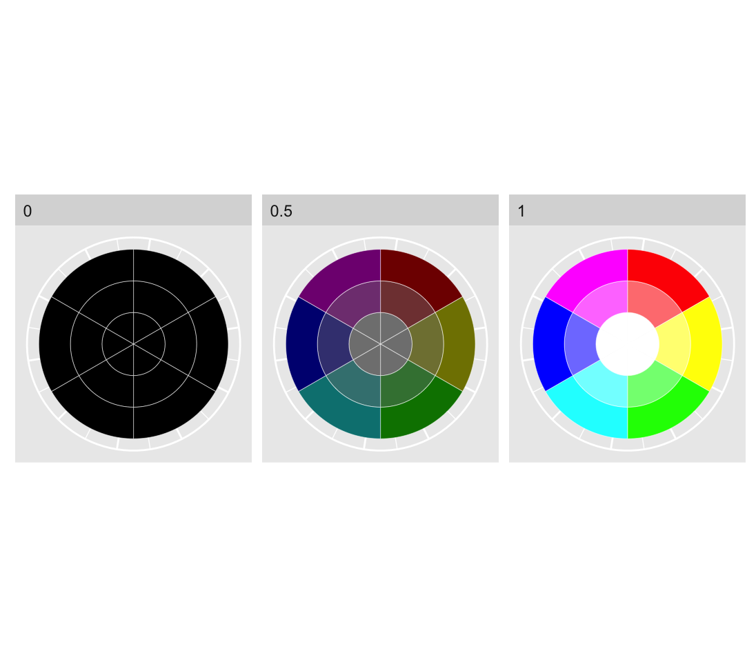
In fig. Figure fig-HSVColSpaceSimple we have the three primary colors (red, green and blue) and the three secondary colors (magenta, yellow and cyan) composed of even mixtures of primary colors.1
1 Note that the secondary colors in RBG color space correspond roughly to the primary colors in CMYK color space and vice versa.
Figure 1: HSV color definitions for the primary and secondary additive colors. From left to right, lightness of 0, 0.5 and 1. Each pie chart begins with saturation of 0 in the center, 0.5 in the middle and 1 in the outer ring.
Each pie chart in Figure fig-HSVColSpaceSimple reveals that as saturation decreases, different hues converge on a monochrome spectrum from black to white. As lightness increases the colors become brighter, and as saturation decreases the colors become less pure, converging on white, for high lightness, grey for mid lightness and black for low lightness. This is why we won’t encode information with saturation. Very low saturation colors are difficult to distinguish from each other. So that leaves us with hue and lightness. Very dark colors are also difficult to distinguish, so we should use them with caution.
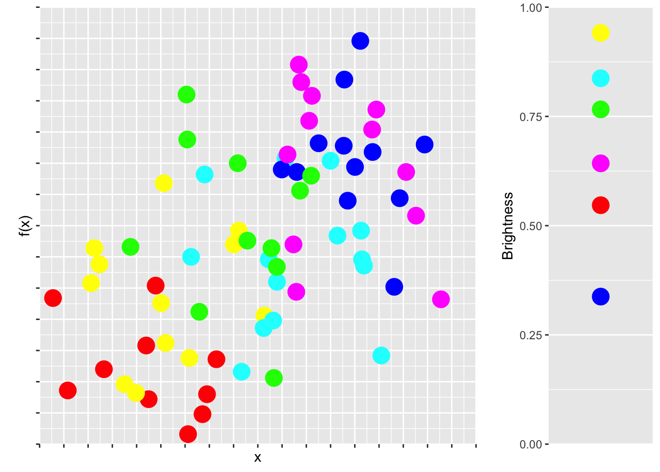
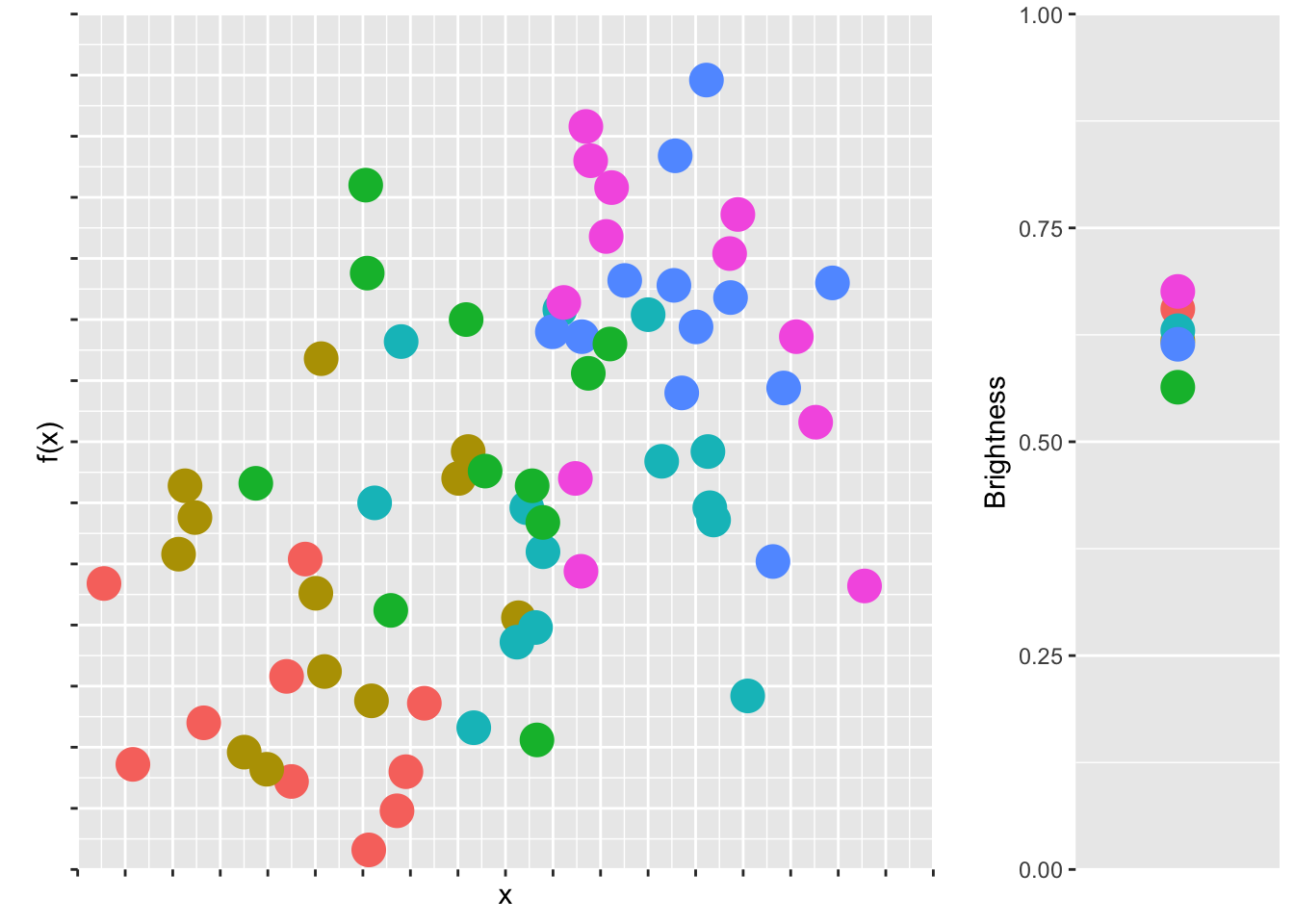
In Figure fig-cheapcol we have a scatter plot of some play data with six disparate colors, each having a high lightness value.
Figure 2: Although very distinct, pure colors are unplesant to look at. In this play data set, the dots are draw with no transparency.
There are couple reasons why the plot in Figure fig-cheapcol doesn’t look very nice. First, the colors are very jarring. High saturation, high lightness colors are just not nice to look at. They kinds of remind us of children’s play rooms. Second, and more subtly, pure colors tend to have cultural meanings. Think of red as a warning color, or yellow for cheapness, or the logos of discount brands. Aldi and Lidl are trying to say something with their color choices!
Third, the main reason why Figure fig-cheapcol doesn’t look good is because the colors, although equally spaced along the color wheel, do not have the same brightness. Brightness refers to the way colors are perceived by our eyes. A bright color appears to emit more light, even if it’s the same lightness in the color space. Brightness can be measured as \(brightness = \sqrt{0.299R^2 + 0.587G^2 + 0.114B^2}\), which means that yellow appears as very bright and blue appears as very dark. The brightness of our six colors is depicted in Figure fig-cheapcol, right.
So this is a perception problem, because colors that are equidistant on the color wheel are not perceived as such by our eyes. They should look great together, but they don’t.2
2 On top of the perception problem, really bright colors cause problems with cheap projectors. Pure yellow or cyan appears faintly, or not at all!
So what is the solution? There have been a few attempts to standardize and make the RBG color space more intuitive. One of the most popular models is the Hue Saturation Value (HSV) (or the Hue Saturation Brightness (HSB)) color space. Here, a color can be specified using three values: hue, saturation, and value (brightness), all in the range of [0, 1]. This is what we saw in the color wheels in Figure fig-HSVColSpaceSimple. As we just saw with our little play example, HSV color space distorts data when used for visualization so that the distance between perceived colors does not reflect their distance in the actual color space.
The Hue Chroma Luminance (HCL) color space solves this problem. HCL color space is like HSV except for one very important distinction: changes in the hue do not effect the lightness. In HCL color space, the perceived difference between two colors is proportional to their Euclidean distance in color space, i.e. we have perceptual uniformity. That makes HCL colors ideal for accurate visual encoding of data. Good news for us!
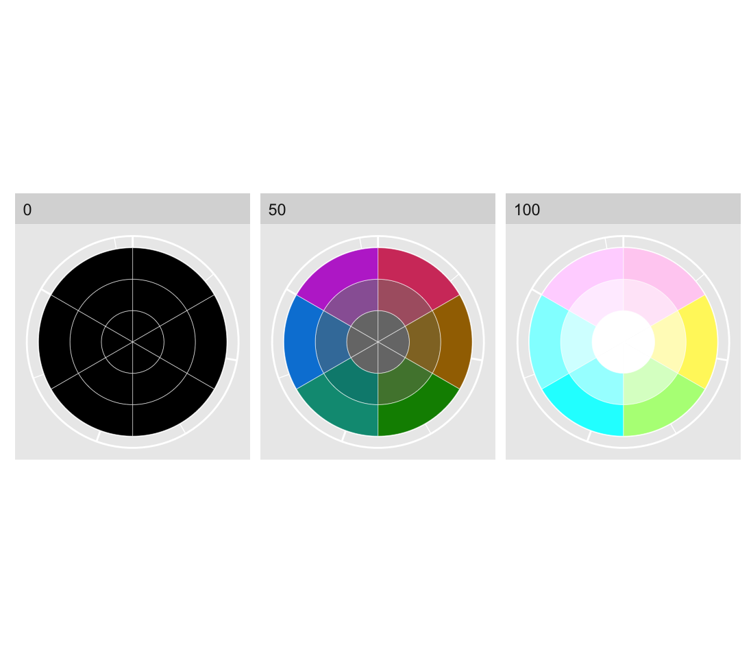
Here, a color can be specified using three values: hue [0, 360], chroma [0, 100]3, and luminescence [0,100]. The HCL color space is designed to match with human visual perception of color in that steps of equal size correspond to approximately equal perceptual changes in color.4
3 Chroma corresponds to saturation.
4 The HSV and HSL color spaces are more intuitive translations of the RGB color space, since they provide a single hue number, either [0, 1] or [0, 360].
Figure 3: HCL color space. The possible values of chroma and luminance depend on the specific hue. The ranges presented here are only indicative.
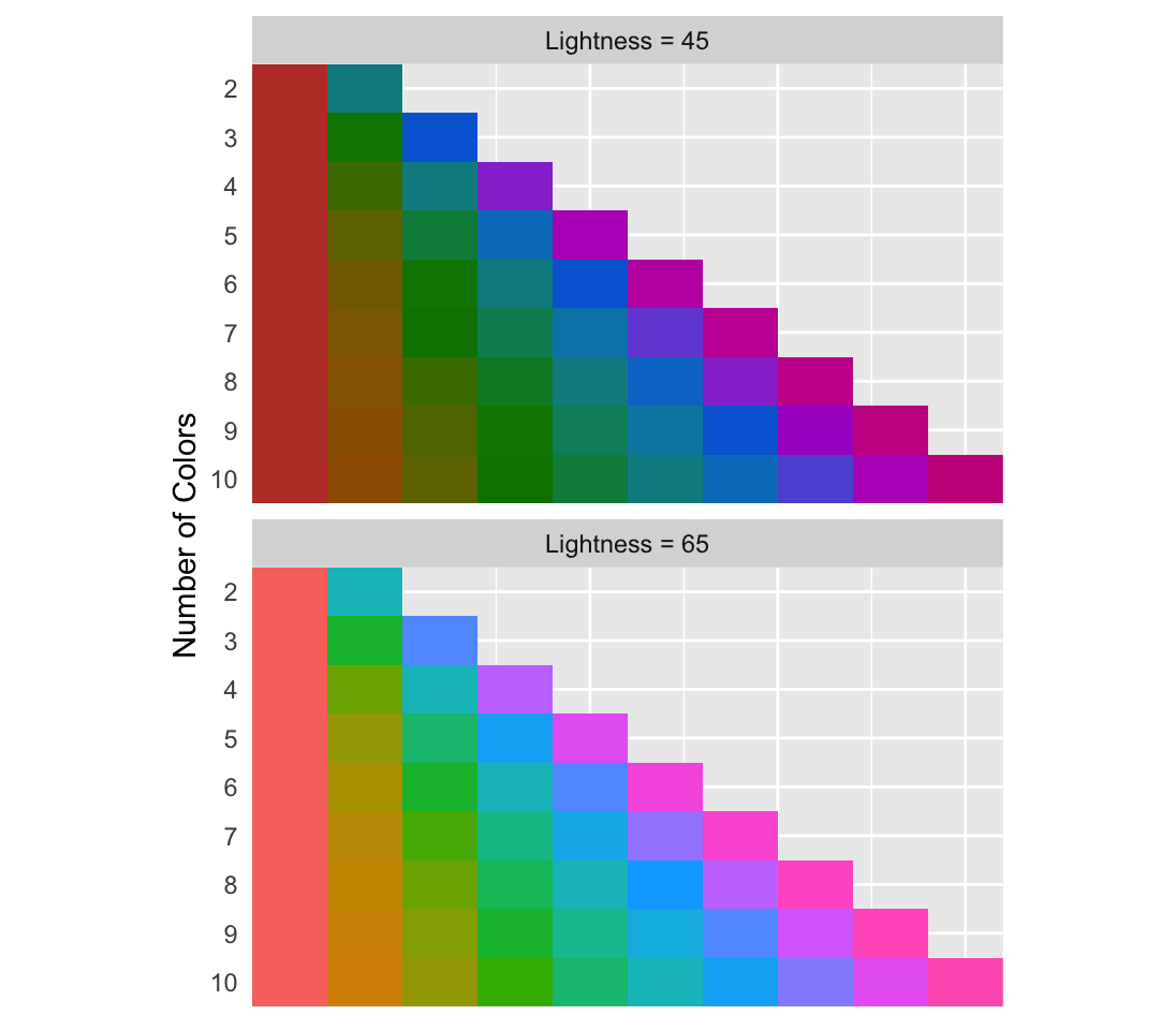
Now, distinct colors can be chosen by evenly spacing them around an HCL color wheel. Two colors will be separated by 180°, three colors by 120° and so on. In Figure fig-ggplotDefault, a chroma of 100 and luminosity of 45 and 65 is used to keep the saturation and lightness consistent while selecting from 2 up to 10 evenly spaced colors.
Figure 4: Evenly spaced colors on the HCL color space.
The default colors used in the R plotting package ggplot2 use an HCL color space with a lightness of 65 and chroma of 100. If you are going to use high saturation, decrease the lightness to avoid blaring colors. Let’s see how the brightness compares now:
Figure 5: A more suitable color scale for our play scatter plot.
The variance of the brightness among the HCL colors is much lower than what we had previously. So if we’re looking for colors that look good together starting with similar brightness helps. However, that doesn’t necessarily mean that the colors will be beautiful or meaningful.
Beautiful colors are subject to fads and trends. What’s beautiful now is hideous in ten years later. If you want to have the nicest color palettes, and don’t have a feeling for choosing colors that work, my best advice is simply to search for “best color palettes” of what ever year you’re in. There is a segment of designers who take joy in developing trendy color palettes and sharing them, so use them to your advantage. A great source is canva.
Barnett, Adrian, and Nicole White. 2024. “Something is off-base with this title: P esteems, statical significance and more slapdash stats.”Significance 21 (1): 11–13. https://doi.org/10.1093/jrssig/qmae007.
Bjork, Robert A, and Elizabeth L Bjork. 2011. “Making Things Hard on Yourself, but in a Good Way: Creating Desirable Difficulties to Enhance Learning.” In Psychology and the Real World: Essays Illustrating Fundamental Contributions to Society, edited by Morton A Gernsbacher, Robert W Pew, Leah M Hough, and James R Pomerantz, 56–64. Worth Publishers.
Briscoe, M. H. 2012. Preparing Scientific Illustrations: A Guide to Better Posters, Presentations, and Publications. Springer New York. https://books.google.de/books?id=mYTlBwAAQBAJ.
Cepeda, Nicholas J, Harold Pashler, Edward Vul, John T Wixted, and Doug Rohrer. 2006. “Distributed Practice in Verbal Recall Tasks: A Review and Quantitative Synthesis.”Psychological Bulletin 132 (3): 354–80.
Chasson, Gregory, and Sara R. Jarosiewicz. 2014. “Social Competence Impairments in Autism Spectrum Disorders.” In Comprehensive Guide to Autism, edited by Vinood B. Patel, Victor R. Preedy, and Colin R. Martin, 1099–1118. New York, NY: Springer New York. https://doi.org/10.1007/978-1-4614-4788-7_60.
Cheeseman, Ian H., Natalia Gomez-Escobar, Celine K. Carret, Alasdair Ivens, Lindsay B. Stewart, Kevin KA Tetteh, and David J. Conway. 2009. “Gene Copy Number Variation Throughout the Plasmodium Falciparum Genome.”BMC Genomics 10 (1): 353. https://doi.org/10.1186/1471-2164-10-353.
Daston, L., and P. Galison. 2007. Objectivity. Book Collections on Project MUSE. Zone Books.
Diemand-Yauman, Connor, Daniel M Oppenheimer, and Erikka B Vaughan. 2011. “Fortune Favors the Bold (and the Italicized): Effects of Disfluency on Educational Outcomes.”Cognition.
Hench, Virginia K., and Lishan Su. 2011. “Regulation of IL-2 Gene Expression by Siva and FOXP3 in Human t Cells.”BMC Immunology 12 (1): 54. https://doi.org/10.1186/1471-2172-12-54.
Hill, Jennifer, and Maria Singer. 2014. “A Comparison of Print and Digital Reading Comprehension by Middle School Students.”Reading Research Quarterly 49 (2): 185–203. https://doi.org/10.1002/rrq.68.
Lupton, E. 2010. Thinking with Type, 2nd Revised and Expanded Edition: A Critical Guide for Designers, Writers, Editors, & Students. Princeton Architectural Press. https://books.google.de/books?id=Y_NVRQAACAAJ.
Mangen, Anne, and Don Kuiken. 2014. “Lost in an iPad: Narrative Engagement on Paper and Tablet.”Scientific Study of Literature 4 (2): 150–77. https://doi.org/10.1075/ssol.4.2.01man.
Mangen, Anne, Bente R Walgermo, and Kolbjørn Brønnick. 2013. “Reading Linear Texts on Paper Versus Computer Screen: Effects on Reading Comprehension.”International Journal of Educational Research 58: 61–68. https://doi.org/10.1016/j.ijer.2012.12.002.
Margolin, Sara J, Christine Driscoll, Michael J Toland, and Jessica L Kegler. 2013. “E-Readers, Computer Screens, or Paper: Does Reading Comprehension Change Across Media Platforms?”Applied Cognitive Psychology 27 (4): 512–19. https://doi.org/10.1002/acp.2930.
Murayama, Hiroshi, Yusuke Takagi, Hirokazu Tsuda, and Yuri Kato. 2023. “Applying Nudge to Public Health Policy: Practical Examples and Tips for Designing Nudge Interventions.”International Journal of Environmental Research and Public Health. MDPI. https://doi.org/10.3390/ijerph20053962.
producer, Stephen Lambert ;. written executive, and produced by Adam Curtis ;. RDF Television; BBC. [2009?]. “The Century of the Self.” Standard format. Wyandotte, MI : BigD Productions, [2009?]. https://search.library.wisc.edu/catalog/9910135083802121.
Roediger, Henry L, and Jeffrey D Karpicke. 2006. “Test-Enhanced Learning: Taking Memory Tests Improves Long-Term Retention.”Psychological Science 17 (3): 249–55.
Rohrer, Doug, and Kelli Taylor. 2007. “The Shuffling of Mathematics Problems Improves Learning.”Instructional Science 35 (6): 481–98.
Roßa, N. 2017. Sketchnotes: Visuelle Notizen für Alles. frechverlag.
———. 2020. Sketchnotes: Die Große Symbol-Bibliothek. frechverlag.
Rousselet, Guillaume A, John J Foxe, and J Paul Bolam. 2016. “A Few Simple Steps to Improve the Description of Group Results in Neuroscience.”Eur. J. Neurosci. 44 (9): 2647–51.
Sanges, Remo, Yavor Hadzhiev, Marion Gueroult-Bellone, Agnes Roure, Marco Ferg, Nicola Meola, Gabriele Amore, et al. 2013. “Highly conserved elements discovered in vertebrates are present in non-syntenic loci of tunicates, act as enhancers and can be transcribed during development.”Nucleic Acids Research 41 (6): 3600–3618. https://doi.org/10.1093/nar/gkt030.
Singer, Leona M, Patricia A Alexander, and Deborah D Reese. 2014. “Reading on Paper and Digitally: What the Past Decades of Empirical Research Reveal.”Review of Educational Research 84 (4): 509–45. https://doi.org/10.3102/0034654314541101.
Slamecka, Norman J, and Peter Graf. 1978. “The Generation Effect: Delineation of a Phenomenon.”Journal of Experimental Psychology: Human Learning and Memory 4 (6): 592–604.
“Status of Mind - social media and young people’s mental health and wellbeing.” 2017. Royal Society for Public Health.
Wästlund, Erik, Lars Nilsson, and Kenneth Holmqvist. 2012. “Eye Movement Patterns and Reading Processes in Eye-Friendly and Non-Eye-Friendly Typography.”Information Design Journal 19 (2): 119–32.